Counting the periods until the amplitude is reduced to a half on a Q = 30 tank circuit.
Resonance is a very common phenomenon, especially in electronics, acoustics, mechanics and optics. When a resonance is desired, special devices are built, called resonators, that have the property of naturally oscillating at some frequency, called resonant frequency, with (much) greater amplitude than at others.
All resonators are characterized by their resonant frequency f0 and their quality factor Q: this page is about a simple method of measuring Q, called the ring-down method.
In electronics, LC circuits are a common kind of resonator, often called resonant circuit, tuned circuit or tank circuit. They are all composed by an inductor (labelled L) and a capacitor (labelled C) connected together. The resistor (labelled R) is responsible for the losses and the final Q-factor: it's often ignored or omitted and rarely added as a physical component, but always present as any losses in the resonator will appear as a resistor. So, every practical LC circuit is actually an RLC circuit, even if just called LC, as it's also the case in this page. Usually, the inductor is responsible for the majority of the losses.
This page is mainly oriented on electrical LC circuits, but the ring-down method applies to all kinds resonator, because the equations describing their behavior have the same form.
Some resonators, like cavities, or vibrations in a metal plate, usually have more than one resonance: in this case, the ring-down method only works if one resonance is much stronger than the others or, in other words, if the other resonances can be neglected. This is true, for example, for tuning forks, but not so much for cavities or delay lines.
The quality factor Q can be defined in many different ways, but here it's good to think about it as the ratio between the total energy in the resonator and the energy lost at each cycle, multiplied by 2π. So, at every oscillation some energy is lost and Q describes the "smallness" of these losses. A resonator that loses very little energy at each cycle has a high Q and will keep oscillating for a long time. Another resonator with higher losses will have a lower Q and its oscillation will die out faster. The ring-down method is a way of measuring Q by measuring the time it takes to the amplitude do decrease by a half. By the way, the percentage of amplitude loss at each cycle is always the same, regardless of the absolute amplitude.
The ring-down method is extremely simple: first you have to "shake" the resonator someway to make it oscillate at its natural frequency. Then, while observing the amplitude of the oscillations decrease, count how many cycles it takes to halve the amplitude and multiply this number by 4.53 to find Q.
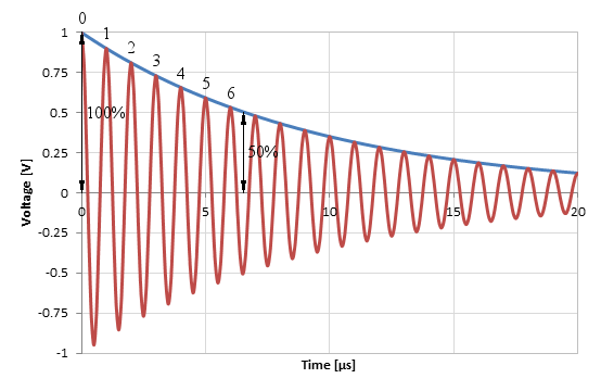
The following plot shows an example: the red line is the signal of the resonator, the blue line is its envelope. Of course, you won't see the envelope line on an oscilloscope, but it quite easy to imagine it by looking at the signal, as the envelope represents the amplitude of the oscillations.
Counting the periods until the amplitude is reduced to a half on a
Q = 30 tank circuit.
Here, we take our 100% reference at t = 0 and we see that it takes about 6.5 cycles for the amplitude to drop by 50%. Simply by doing 6.5 · 4.53 we find Q ≅ 30.
You don't need to start counting from the very first oscillation: pick any cycle you want, as it will always take the same amount of cycles for the amplitude to decrease by the same factor.
This method looks really simple, and indeed it is, but you need to be careful: what you're measuring is the total Q-factor of the resonator degraded by the additional losses introduced by the method you use to measure the oscillation amplitude (the oscilloscope, for example) and the ones due to the way you "shake" the resonator. The Q-factor of the resonator alone will always be higher. It's important to wisely choose your setup to minimize these additional losses. This usually translates into coupling the test instruments as loose as possible to the resonator while still having enough signal for a reliable measurement. More on this below.
Now, if you don't need high precision, and Q rarely needs to be very accurate, you can approximate 4.53 to 5. Counting some oscillations on a screen and multiplying by 5 is something you can quickly do in hour head without the need of a calculator. In my opinion, this is the beauty of this method: you can just watch at a waveform on your oscilloscope and directly "see" the Q-factor.
The ring-down method is so simple that I often wondered how it works: so, let's dig into it. We start by assuming that the resonator can be described with a simple linear homogeneous differential equation of order 2, as it's usually the case. The general solution of this equation has the form:
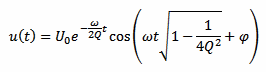
Often, in this equation, the square root is omitted, because for a large Q, this square root almost equals one; and resonators do have a large Q. Without the square root, the cosine term is just cos(ωt+φ) that looks much more familiar. U0 and φ are constants.
Here, I wrote u(t) because I was thinking of a voltage, but this really doesn't matter: it could be a pressure, a displacement or whatever.
The above equation is written in terms of Q and ω, as they includes all the important parameters of the resonator.
For example, for LC electrical circuits, Q is expressed as follows (for parallel and series circuits respectively):
 ;
;

The pulsation ω is defined as 2πf, where f is the frequency. For LC circuits (series or parallel), ω is defined as follows:

Again, this is just to place the resonator equation in a context: any resonator having characteristics similar to u(t) will have its own Q and ω but will behave in the same way.
If we plot this equation we obtain the following curve, where we can observe the damped oscillations and the exponentially decreasing envelope:
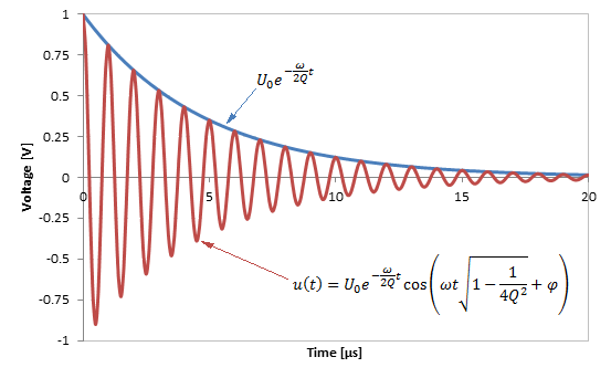
The damped oscillation and its equation.
You may notice that this equation has two parts: a an exponential and a cosine. The cosine alone has an amplitude which is always between –1 and +1. The overall amplitude is therefore controlled by the exponential term (including the constant U0), which is called the envelope. When we look at the amplitude of the oscillations, we are actually interested in the amplitude of the envelope, the amplitude of the cosine is well known and not relevant for our purpose.
We want to prove "magic recipe" of the ring-down method, which is simply:

Let's start by finding the time t when (the envelope of) u(t) is half of what it was at the beginning, u(0):

By replacing u(t) with the envelope part of our first equation we have:
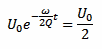
As explained before, we don't care about the cos() term of u(t) whose amplitude is always between –1 and +1; we only care about the envelope part of u(t), which is U0e–(ωt/2Q).
Now, U0 cancels out:

By taking the natural logarithm, we obtain:
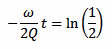
Now we get rid of the minus sign and we find:

This equation still has the time t in it, while we want to deal with the number of cycles N. For this, we consider that the pulsation ω is defined as follows, where T is the period of the oscillation:

We consider also that the number of cycles N of period T that happen in the time t is just:

By putting all together, we find:
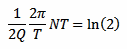
Now, T cancels out leaving:

That we can solve for Q:
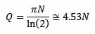
This is the result we were looking for, and it's interesting to remark that any dependency in ω, t, T, U0 and φ disappeared: Q depends only on N.
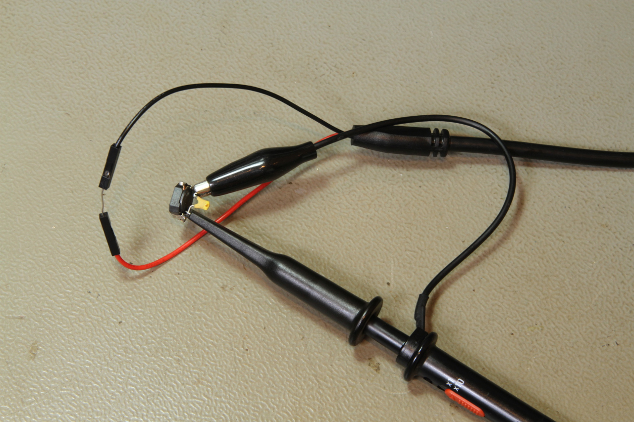
Even if the ring-down method applies to almost any resonator, LC tank circuits are very common in RF engineering: I think it's worth spending a few words about how to measure them. Two external instruments need to be connected: some sort of signal generator to "shake" (maybe "tickle" is a batter word) the resonator and most probably an oscilloscope to measure the signal amplitude. In both cases, it's important to use as little coupling as possible, because coupling will load the resonator and decrease its Q-factor.
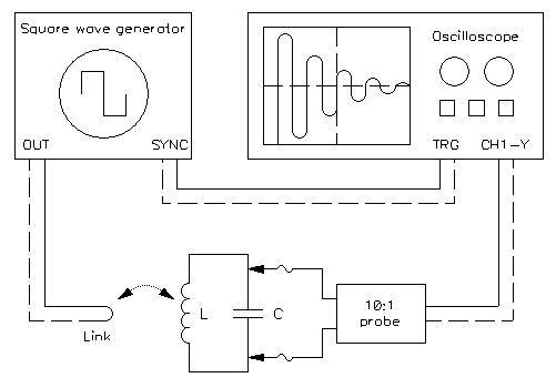
A possible connection of the LC tank circuit under test to the square
wave generator and to the oscilloscope.
My favorite test setup is shown in the above picture. A square wave generator is used to shake the tank via a loose inductive coupling while an oscilloscope is connected to the resonator via a 10:1 probe. The scope is synchronized to the generator with a dedicated cable: this is not strictly required, but greatly simplifies the operation of stabilizing the image on the screen. If you have a digital oscilloscope, you can acquire the data with just a single pulse, but for analog scopes, a square wave produces a nice and steady image.
The square wave generator is run at a much lower frequency than the resonance of the tank. For example, a few kHz are fine for resonators in the MHz to many MHz range. The exact value of it is not important: it just has to be much much lower. In other words, the induced oscillation should have the time to be damped away (almost completely) before the next edge comes in (this just produces better images easier to measure; the method work regardless of the amplitude when the next "kick" comes in).
The square wave must have very fast rising and falling edges: it must change state much faster than the period of oscillation of the tank. Every edge of the wave will give a nice "kick" to the tank. Laboratory signal generators are usually fine. If you don't have one, you can easily build one with a TTL (7400 series) or HCTTL (74HC00 series) IC, or with any other suitable fast logic IC. For this, unfortunately, the good old 555 IC is too slow and the edges are not fast enough. Make sure your generator can handle a short circuit on its output: if not, connect a series resistor (47 Ω or so).
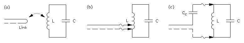
Various methods of connecting the square wave generator to the tank
circuit: (a) loose inductive coupling, (b) autotransformer coupling and (c)
weak capacitive coupling.
The signal generator can be connected in several different ways. My preferred is with a loose inductive coupling as shown in the (a) part of the above diagram. This is basically a wire loop shorting the output placed near the resonator. The advantage is that it's extremely easy to change the coupling and find the best compromise just by moving the loop.
An alternative method is using the inductor of the resonator as a step-up transformer as shown in (b), but you need to have access to the inductor winding which, in some cases, may be quite difficult. Then, for changing the coupling, you need to tap at a different point of the coil and can be quite tricky as well, especially in small inductors.
Capacitive coupling shown in (c) also works quite well, but requires an extra capacitor Cc. The smallest the capacitor the looser the coupling. For changing the coupling you need to change the capacitor (or use a capacitive trimmer). For the MHz range, use 1 pF as starting point. The capacitance required is very small: for VHF or higher frequencies, just placing the cable end at a few mm from the resonator may introduce just enough stray capacitance that no real coupling capacitor is needed.
To replace the square wave, I once tried the spark produced by a piezo lighter fired nearby to kick the resonator, but this wasn't a good idea: it somehow works in kicking the oscillations, but it's so noisy that the measurements are almost useless.
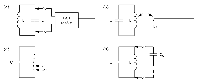
Various methods of connecting the oscilloscope to the tank circuit:
(a) direct high-impedance probe connection, (b) loose inductive coupling, (c)
autotransformer coupling and (d) weak capacitive coupling.
For connecting an instrument for measuring the amplitude, the same methods explained before also work fine. They are shown in (b), (c) and (d) of the above picture. But if you want to connect an oscilloscope, I still prefer method (a) where you just connect it in parallel to the tank. This only works with oscilloscopes, because of their high input impedance. If you want to connect a low impedance instrument, a wattmeter with 50 Ω impedance for example, method (a) will not work; but (b), (c) or (d) will do fine.
The usual input impedance if a scope is 1 MΩ: it's high but not very high. Connecting it directly to a tank often works, but may be an issue for high-Q resonators where this extra MΩ will significantly affect the Q-factor. I prefer using a 10:1 probe: it has an input impedance of 10 MΩ and loads the tank 10 times less at the cost of a 10 times smaller signal on the screen. 10:1 probes also have a much smaller stray capacitance, but this is only important if you also want to calculate L or C by observing the period of the oscillations.
If in doubt about loading too much your resonator, just connect an extra resistor in parallel to it of about the same value of the input impedance of your probe: if you see that the damping increases (the oscillation dies out faster), than you're loading too much and you should reduce the coupling. To do this, you can go for another coupling method such as (b), (c) or (d) that you can also use with a 10:1 probe for reducing the coupling even more.
If the resonator under test is already installed in a circuit, with input and output connections already in place, it's worth considering reusing these connections for the measurement (and related amplifiers, if present), so that no additional loading is added. In this case, impedance matching may be an issue.
Let's have a look at a few examples to see how this method works. First let's take a small ferrite inductor and connect it in parallel to a ceramic capacitor. The inductor measures 2.56 μH and the capacitor 448 pF (the resonance frequency is therefore 4.700 MHz corresponding to a period of 213 ns). The test setup is visible in the picture below, where the loop connects to the square wave generator and the oscilloscope is connected in parallel with the LC circuit with a 10:1 voltage probe. Because the inductor is shielded, the coupling loop needs to be quite close to the tank circuit in order to have some coupling.
A small ferrite 2.56 μH inductor and a ceramic 448 pF
capacitor being tested with the ring-down method.
The square wave generator is connected to the loop and the oscilloscope is in
parallel via a 10:1 probe (click to enlarge).
The square wave generator is set at about 2 kHz and the oscilloscope is synchronized with it. The waveform is visible in the picture below:
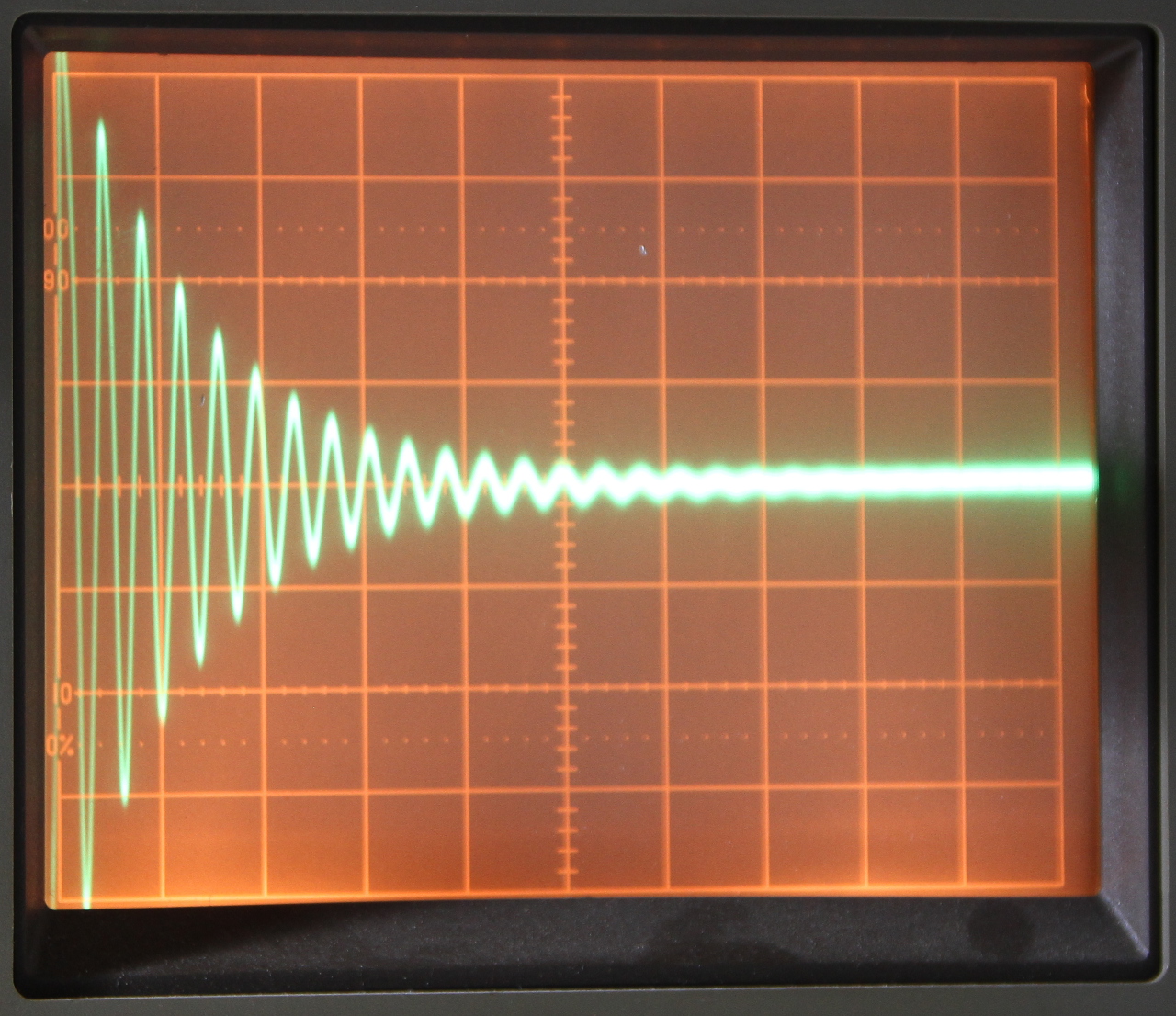
Ring-down signal of the circuit. 10 mV/DIV, 0.5 μs/DIV.
The amplitude of the signals halves in about 2.5 cycles, the Q-factor is
therefore 11.3 (click to enlarge).
As you can see, the amplitude of the signals halves in about 2.5 cycles and we can easily calculate the Q-factor by multiplying by 4.53 and we find Q = 11.3.
The Q-factor of this tank is not very good: 11.4 is quite low, but it's not surprising. Small inductors like this one are mainly intended for switching power supplies and generally have a Q-factor between 10 and 20, only some expensive and rare models may reach 40. The ceramic capacitor used here is good for high frequency applications and does not (negatively) influence the Q-factor.
Let's do the same test with a better inductor. Here I took an air core inductor made with thick copper wire (pipe) that measures 2.05 μH (not exactly the same inductance as before but close enough) and a high voltage ceramic capacitor measuring 490 pF (the resonance frequency is therefore 5.022 MHz corresponding to a period of 199 ns). These components are designed for building high power transmitters: they handle high power with very little losses. The inductor is composed by 8 turn of Ø8 mm copper tubing winded on a Ø62 mm internal diameter air core. The coil pitch is 14 mm.
The test setup is visible in the picture below, where the loop connects to the square wave generator and the oscilloscope is connected in parallel with the LC circuit with a 10:1 voltage probe. The position of the loop has been adjusted until the desired coupling has been achieved: in this case, quite far from the inductor because the air core configuration ensures a much better coupling than before.
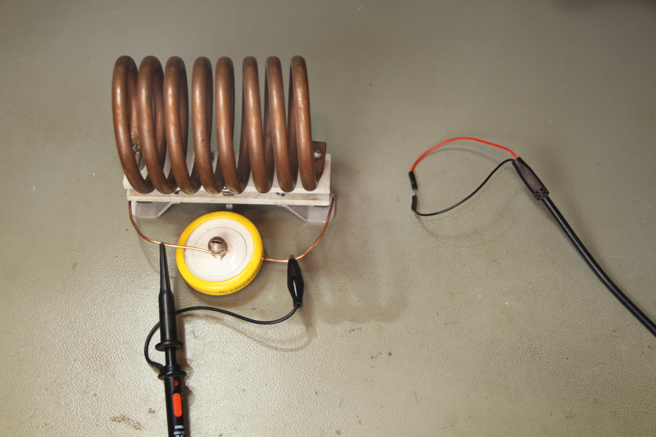
A big air core 2.05 μH inductor and a high voltage ceramic
490 pF capacitor being tested with the ring-down method.
The square wave generator is connected to the loop and the oscilloscope is in
parallel via a 10:1 probe (click to enlarge).
As before, the square wave generator is set at about 2 kHz and the oscilloscope is synchronized with it. The resulting waveform is visible in the picture below:
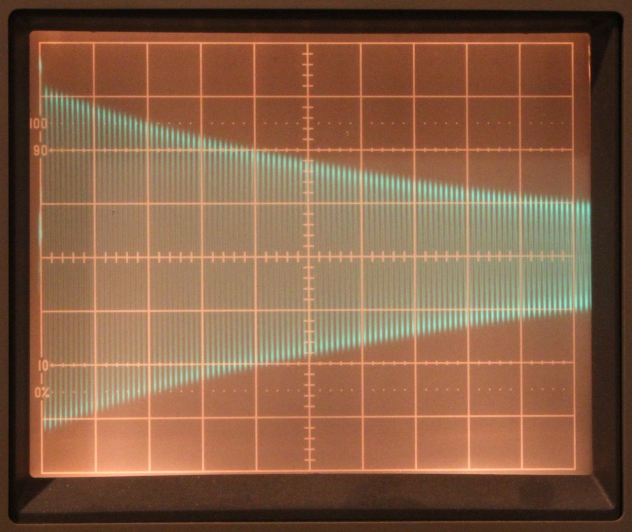
Ring-down signal of the circuit. 10 mV/DIV, 2 μs/DIV.
The amplitude of the signals halves in about 63 cycles, the Q-factor is
therefore 285 (click to enlarge).
As you can see, the amplitude of the signal decreases much more slowly and halves in about 63 cycles. We can easily calculate the Q-factor by multiplying by 4.53 and we find Q = 285. This is a very good quality factor: good inductors are usually around 250, but the price to pay is the bigger size and the large amount of precious copper (and sometimes silver) required to build them.
Just for fun, let's have a look at an even better LC resonant circuit: a magnetic loop antenna. The one represented in the picture below is composed by 2 turns of Ø18 mm copper pipe on a Ø95 cm air core. The coil pitch is 40 mm and measures 7.4 μH. It's tuned to 1.850 MHz with a 1.0 nF vacuum capacitor.
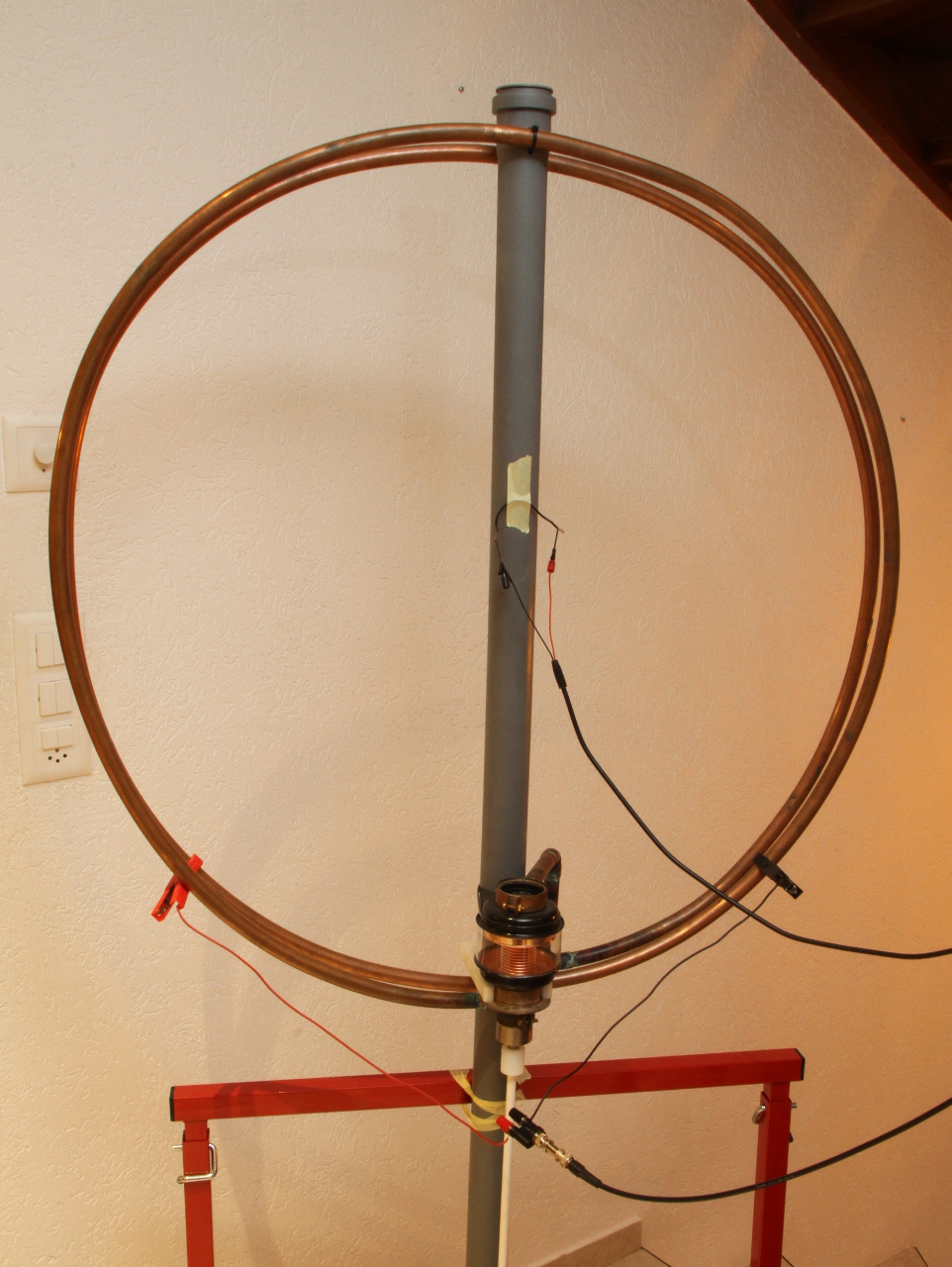
A magnetic loop antenna tuned at 1.850 MHz being tested with the
ring-down method.
The square wave generator is connected to the small loop in the middle and
the oscilloscope is directly connected via the two clamps (click to
enlarge).
The square wave generator is set at about 1 kHz here and the oscilloscope is synchronized with it. To avoid damping this very high Q-factor resonator, the oscilloscope is directly connected via the two clamps (method (c) explained before), as the direct connection of the 10:1 probe would have slightly loaded the tank. The square wave generator is connected to the small loop in the middle. The resulting waveform is visible in the plot below:
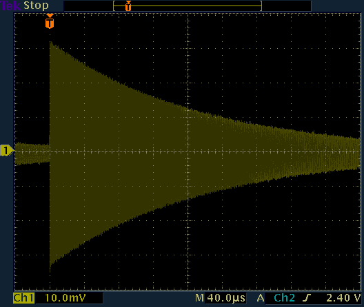
Ring-down signal of the antenna.
The amplitude of the signals halves in about 116 μs, which represents
215 cycles at 1.850 MHz: the Q-factor is therefore 970 (click to enlarge).
Here, the Q-factor is so high that it's not possible to directly observe and count the cycles anymore. But we can see that it takes 116 μs for the amplitude to decrease to a half. At 1.850 MHz, there are 215 cycles in 116 μs (as a reminder, 116 μs · 1.850 MHz = 215 cycles). The quality factor can therefore be obtained as usual by multiplying 215 by 4.53 and we find Q = 972. This is an extremely good quality factor for an inductor based resonant circuit, mainly due to the large amount of copper used in the coil.
All the previous examples were electrical circuits. Let's have a look now at a mechanical resonator, as the ring-down method applies to almost any resonator. I choose a 440 Hz tuning fork used by guitar players to tune their instrument. To measure the amplitude of the oscillations it has been coupled to a piezoelectric transducer and connected to the oscilloscope, as shown in the picture below. The piezoelectric transducer works here as a microphone. Here, the choice of the probe is not important, but the way to hold the fork in place is critical: I ended up tying it to a long wooden stick with thin copper wire, being careful in not tightening it too much.
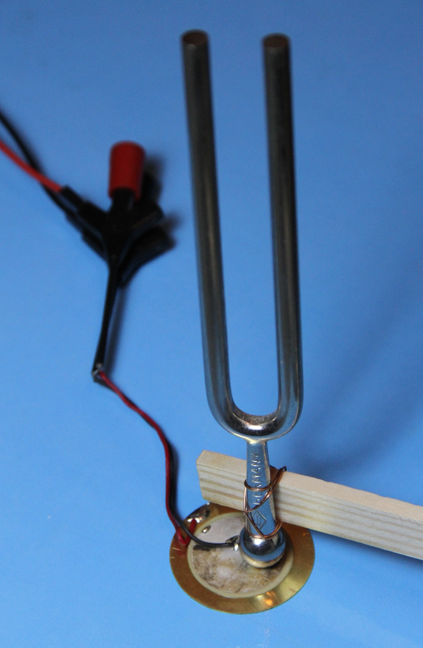
A 440 Hz tuning fork mounted on a piezoelectric transducer and
being tested with the ring-down method (click to enlarge).
Here, no square wave generator is used; I just gently hit the top of the fork with the handle of a screwdriver. Since this is a "one time" operation, it's much easier to do with a digital oscilloscope that can record a single event. The result is shown in the following plot:
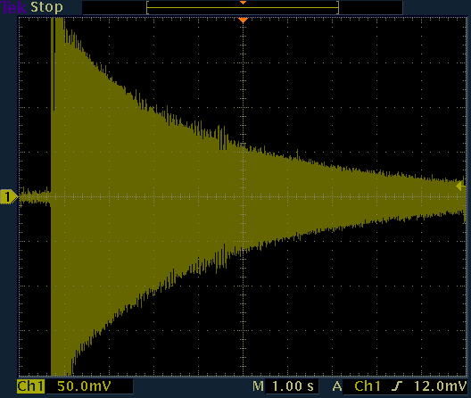
Ring-down signal of the tuning fork.
The amplitude of the signals halves in about 2.4 s, which represents
about 1060 cycles at 440 Hz: the Q-factor is therefore 4800 (click to
enlarge).
Again, the Q-factor is so high that it's not possible to directly observe and count the cycles. There is some noise on the signal, picked up by the microphone while measuring, but we see that it takes 2.4 s for the amplitude to decrease to a half. At 440 Hz, there are about 1060 cycles in 2.4 s and the quality factor is Q = 4800. This is not surprising at all: when we strike a tuning fork, we hear its tone for quite a long time (many seconds): it must have a very high quality factor. Please remark that because of the noise, it's not worth calculating Q with too many significant digits.
The ring-down method for determining the Q-factor of a resonator has been described, illustrated and commented. It can simply be resumed in counting how may cycles it takes to halve the amplitude of the oscillations and multiplying this number by 4.53. It's a very handy method that basically requires just an oscilloscope and some minor extra equipment. Personally, it's my preferred method and I find it simple and practical in many situations.
If you're not obsessed by precision, you can simply multiply by 5 instead of 4.53 and you won't even need a calculator: you can deduce Q simply by looking at your old analog oscilloscope screen.
| [1] | Hans Nussbaum, DJ1UGA. HF-Messungen für den Funkamateur, Teil 1. Verlag für Technik und Handwerk Funk-Fachbuch, 2. Auflage, 2006, Seiten 58-61. |
| [2] | H. Matzinger. Analyse II: Cours du Prof. H. Matzinger. École Polytechniques Fédérale de Lausanne, 1994/95, Chapter XI.2. |
| [3] | A. Germond. Electrotechnique, Support du cours du Prof. A. Germond. Chapitre 2, Enclenchements et déclenchements sur sources de tensions ou de courants continus. École Polytechniques Fédérale de Lausanne, 1995. |
| Home | Electronics | Page hits: 101972 | Created: 12.2014 | Last update: 12.2014 |